Off-Axis Field of a Current Loop¶

This simple formula can be obtained using the Law of Biot Savart, integrated over a circular current loop to obrtain the magnetic field at any point in space. Compare this to the much simpler formula for calculating the on-axis magnetic field due to a current loop.

Magnetic field in vicinity of a current loop. Point is located at axial distance, x, and radius, r.

Axial, Radial Components¶

$B_x = B_0 \frac 1 {\pi \sqrt Q} \left[E(k) \frac {1-\alpha^2-\beta^2}{Q-4\alpha} + K(k) \right]$

$B_r = B_0 \frac {\gamma} {\pi \sqrt Q} \left[E(k) \frac {1+\alpha^2+\beta^2}{Q-4\alpha} - K(k) \right]$

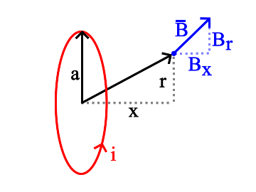
$B$ is the magnetic field (Tesla) at any point in space that isn't on the current loop. It is equal to the sum of two field components: $B_x$ the field component that is aligned with the axis and $B_r$, the field component that is in a radial direction. Symbols are defined:

$\alpha = \frac r a $ and $\beta = \frac x a $ and $\gamma = \frac x r$

$Q = \left[\left(1 + \alpha\right)^2 + \beta^2 \right]$

$k = \sqrt {\frac {4 \alpha} Q}$

$B_0$ is the magnetic field at the center of the coil: $B_0 = \frac {i \mu_0} {2a}$

$i$ is the current in the loop wire (Amperes)

$a$ is the loop radius (meters)

$\mu_0$ is the permeability constant (approx. 1.26 x 10^-6 or exactly π4 x 10^-7)

$x$ is the distance in the axial direction from the center of the current loop to the field measurement point.

$r$ is the distance in the radial direction from the axis of the current loop to the field measurement point.

$K(k)$ is the complete elliptic integral function, of the first kind

$E(k)$ is the complete elliptic integral function, of the second kind.

Please take note that not all software computes complete elliptic integrals using the same notation. For example, the scipy ellipe function accepts the parameter $m$ instead of $k$. See the example code below, and this discussion of notational variants for more information.

Online Calculator¶

Please see the online calculator for finding fields at any point in space due to a current loop.

Example Application¶

The following Python code implements the formulas on this page and presents curves that show axial and radial field strength components in the vicinity of a 1m radius loop of wire carrying 1A of current.

Credits¶

Formulas on this page are adapted from SOME USEFUL INFORMATION FOR THE DESIGN OF AIR-CORE SOLENOIDS by D. Bruce Montgomery and J. Terrell.

%matplotlib inline
from scipy.special import ellipk, ellipe, ellipkm1
from numpy import pi, sqrt, linspace
from pylab import plot, xlabel, ylabel, suptitle, legend, show

uo = 4E-7*pi     # Permeability constant - units of H/m
Bo = lambda i, a, u=uo: i*u/2./a    # Central field = f(current, loop radius, perm. constant)
al = lambda r, a: r/a               # Alpha = f(radius of measurement point, radius of loop)
be = lambda x, a: x/a               # Beta = f(axial distance to meas. point, radius of loop)
ga = lambda x, r: x/r               # Gamma = f(axial distance, radius to meas. point)
Q = lambda r, x, a: (1 + al(r,a))**2 + be(x,a)**2   # Q = f(radius, distance to meas. point, loop radius)
k = lambda r, x, a: sqrt(4*al(r,a)/Q(r,x,a))       # k = f(radius, distance to meas. point, loop radius)
K = lambda k: ellipk(k**2.0)          # Elliptic integral, first kind, as a function of k
E = lambda k: ellipe(k**2.0)          # Elliptic integral, second kind, as a function of k

# On-Axis field = f(current and radius of loop, x of measurement point)
def Baxial(i, a, x, u=uo):
    if a == 0:
        if x == 0:
            return NaN
        else:
            return 0.0
    else:
        return (u*i*a**2)/2.0/(a**2 + x**2)**(1.5)

# Axial field component = f(current and radius of loop, r and x of meas. point)
def Bx(i, a, x, r):
    if r == 0:
        if x == 0:
            return Bo(i,a)         # central field
        else:
            return Baxial(i,a,x)   # axial field
    else:                          # axial component, any location
        return Bo(i,a)*\
            (E(k(r,x,a))*((1.0-al(r,a)**2-be(x,a)**2)/(Q(r,x,a)-4*al(r,a))) + K(k(r,x,a)))\
            /pi/sqrt(Q(r,x,a))
        
# Radial field component = f(current and radius of loop, r and x of meas. point)
def Br(i, a, x, r):
    if r == 0:
        return 0                   # no radial component on axis!
    else:                          # radial component, any location other than axis.
        return Bo(i,a)*ga(x,r)*\
            (E(k(r,x,a))*((1.0+al(r,a)**2+be(x,a)**2)/(Q(r,x,a)-4*al(r,a))) - K(k(r,x,a)))\
            /pi/sqrt(Q(r,x,a))

Construct a family of field strength curves, as a function of radius and axial distance, for a unit coil (1m radius, 1A current):

axiallimit = 2.0 # meters from center
radiallimit = 0.5 # maximum radius to investigate
curveqty = 5
X = linspace(0,axiallimit)
R = linspace(0, radiallimit, curveqty)
[plot(X, [Bx(1,1,x,r) for x in X], label="r={0}".format(r)) for r in R]
xlabel("Axial Position (m)")
ylabel("Axial B field (T)")
suptitle("Axial component of unit coil (1m radius, 1A current) B field for various measurement radii")
legend()
show()

[plot(X, [Br(1,1,x,r) for x in X], label="r={0}".format(r)) for r in R]
xlabel("Axial Position (m)")
ylabel("Radial B field (T)")
suptitle("Radial component of unit coil (1m radius, 1A current) B field for various measurement radii")
legend()
show()

[plot(X, [sqrt(Bx(1,1,x,r)**2 + Br(1,1,x,r)**2) for x in X], label="r={0}".format(r)) for r in R]
xlabel("Axial Position (m)")
ylabel("B field (T)")
suptitle("Total unit coil (1m radius, 1A current) B field for various measurement radii")
legend()
show()

Now re-examine the nature of the B_r field by plotting families of curves where the horizontal axis is radial position:

R = linspace(0, radiallimit)
X = linspace(0, axiallimit, curveqty)
[plot(R, [Bx(1,1,x,r) for r in R], label="x={0}".format(x)) for x in X]
xlabel("Radial Position (m)")
ylabel("Axial B field (T)")
suptitle("Axial component of unit coil (1m radius, 1A current) B field for various axial positions")
legend()
show()

[plot(R, [Br(1,1,x,r) for r in R], label="x={0}".format(x)) for x in X]
xlabel("Radial Position (m)")
ylabel("Radial B field (T)")
suptitle("Radial component of unit coil (1m radius, 1A current) B field for various axial positions")
legend()
show()

[plot(R, [sqrt(Bx(1,1,x,r)**2+Br(1,1,x,r)**2) for r in R], label="x={0}".format(x)) for x in X]
xlabel("Radial Position (m)")
ylabel("B field (T)")
suptitle("Total unit coil (1m radius, 1A current) B field for various axial positions")
legend()
show()